About 50,000 folks learn my article 3 superior free Math packages. Likelihood is that not less than a few of them downloaded and put in Maxima. If you’re certainly one of them however should not acquainted with CAS (Pc Algebra System) software program, Maxima could seem very difficult and troublesome to make use of, even for the decision of easy highschool or calculus issues. This doesn’t should be the case although, whether or not you might be searching for extra math assets to make use of in your profession or a scholar in an internet bachelor’s diploma in math searching for homework assist, Maxima may be very pleasant and this 10 minute tutorial will get you began instantly. When you’ve acquired the primary steps down, you may at all times lookup the particular operate that you just want, or study extra from Maxima’s official handbook. Alternatively, you should utilize the query mark adopted by a string to acquire in-line documentation (e.g. ? combine). This tutorial takes a sensible strategy, the place easy examples are given to indicate you the right way to compute widespread duties. After all that is simply the tip of the iceberg. Maxima is a lot greater than this, however scratching even simply the floor must be sufficient to get you going. Ultimately you might be solely investing 10 minutes.
Maxima as a calculator
You should utilize Maxima as a quick and dependable calculator whose precision is unfair throughout the limits of your PC’s {hardware}. Maxima expects you to enter a number of instructions and expressions separated by a semicolon character (;), identical to you’d do in lots of programming languages.
(%i1) 9+7;
(%o1) [tex]16[/tex]
(%i2) -17*19;
(%o2) [tex]-323[/tex]
(%i3) 10/2;
(%o3) [tex]5[/tex]
Maxima permits you to discuss with the most recent outcome by means of the % character, and to any earlier enter or output by its respective prompted %i (enter) or %o (output). For instance:
(%i4) % - 10;
(%o4) [tex]-5[/tex]
(%i5) %o1 * 3;
(%o5) [tex]48[/tex]
For the sake of simplicity, any further we’ll omit the numbered enter and output prompts produced by Maxima’s console, and point out the output with a => signal. When the numerator and denominator are each integers, a lowered fraction or an integer worth is returned. These could be evaluated in floating level by utilizing the float operate (or bfloat for large floating level numbers):
8/2;
=> [tex]4[/tex]
8/2.0;
=> [tex]4.0[/tex]
2/6;
=> [tex]displaystyle frac{1}{3}[/tex]
float(1/3);
=> [tex]0.33333333333333[/tex]
1/3.0;
=> [tex]0.33333333333333[/tex]
26/4;
=> [tex]displaystyle frac{13}{2}[/tex]
float(26/4);
=> [tex]6.5[/tex]
As talked about above, huge numbers should not a problem:
13^26;
=> [tex]91733330193268616658399616009[/tex]
13.0^26
=> [tex]displaystyle 9.1733330193268623text{ }10^_{+28}[/tex]
30!;
=> [tex]265252859812191058636308480000000[/tex]
float((7/3)^35);
=> [tex]displaystyle 7.5715969098311943text{ }10^_{+12}[/tex]
Constants and customary features
Here’s a record of widespread constants in Maxima, which you need to be conscious of:
- %e – Euler’s Quantity
- %pi – [tex]displaystyle pi[/tex]
- %phi – the golden imply ([tex]displaystyle frac{1+sqrt{5}}{2}[/tex])
- %i – the imaginary unit ([tex]displaystyle sqrt{-1}[/tex])
- inf – actual constructive infinity ([tex]infty[/tex])
- minf – actual minus infinity ([tex]-infty[/tex])
- infinity – complicated infinity
We are able to use a few of these together with widespread features:
sin(%pi/2) + cos(%pi/3);
=> [tex]displaystyle frac{3}{2}[/tex]
tan(%pi/3) * cot(%pi/3);
=> [tex]1[/tex]
float(sec(%pi/3) + csc(%pi/3));
=> [tex]3.154700538379252[/tex]
sqrt(81);
=> [tex]9[/tex]
log(%e);
=> [tex]1[/tex]
Defining features and variables
Variables could be assigned by means of a colon ‘:’ and features by means of ‘:=’. The next code reveals the right way to use them:
a:7; b:8;
=> [tex]7[/tex]
=> [tex]8[/tex]
sqrt(a^2+b^2);
=> [tex]sqrt{113}[/tex]
f(x):= x^2 -x + 1;
=> [tex]x^2 -x + 1[/tex]
f(3);
=> [tex]7[/tex]
f(a);
=> [tex]43[/tex]
f(b);
=> [tex]57[/tex]
Please notice that Maxima solely gives the pure logarithm operate log. log10 just isn’t out there by default however you may outline it your self as proven under:
log10(x):= log(x)/log(10);
=> [tex]displaystyle log10(x):=frac{log(x)}{log(10)};[/tex]
log10(10)
=> [tex]1[/tex]
Symbolic Calculations
issue allows us to search out the prime factorization of a quantity:
issue(30!);
=> [tex]displaystyle 2^{26},3^{14},5^7,7^4,11^2,13^2,17,19,23,29[/tex]
We are able to additionally issue polynomials:
issue(x^2 + x -6);
=> [tex](x-2)(x+3)[/tex]
And increase them:
increase((x+3)^4);
=> [tex]displaystyle x^4+12,x^3+54,x^2+108,x+81[/tex]
Simplify rational expressions:
ratsimp((x^2-1)/(x+1));
=> [tex]x-1[/tex]
And simplify trigonometric expressions:
trigsimp(2*cos(x)^2 + sin(x)^2);
=> [tex]displaystyle cos ^2x+1[/tex]
Equally, we are able to increase trigonometric expressions:
trigexpand(sin(2*x)+cos(2*x));
=> [tex]displaystyle -sin ^2x+2,cos x,sin x+cos ^2x[/tex]
Please notice that Maxima received’t settle for 2x as a product, it requires you to explicitly specify 2*x. In the event you want to acquire the TeX illustration of a given expression, you should utilize the tex operate:
tex(%);
=> $$-sin ^2x+2,cos x,sin x+cos ^2x$$
Fixing Equations and Methods
We are able to simply remedy equations and methods of equations by means of the operate remedy:
remedy(x^2-4,x);
=> [tex]displaystyle left[ x=-2 , x=2 right][/tex]
%[2]
=> [tex]x=2[/tex]
remedy(x^3=1,x);
=> [tex]displaystyle left[ x={{sqrt{3},i-1}over{2}} , x=-{{sqrt{3},i+1}over{2}}  , x=1 right][/tex]
trigsimp(remedy([cos(x)^2-x=2-sin(x)^2], [x]));
=> [tex]displaystyle left[ x=-1 right][/tex]
remedy([x - 2*y = 14,  x + 3*y = 9],[x,y]);
=> [tex]left[ left[ x=12 , y=-1 right]  proper][/tex]
2D and 3D Plotting
Maxima allows us to plot 2D and 3D graphics, and even a number of features in the identical chart. The features plot2d and plot3d are fairly easy as you may see under. The second (and within the case of plot3d, the third) parameter, is simply the vary of values for x (and y) that outline what portion of the chart will get plotted.
plot2d(x^2-x+3,[x,-10,10]);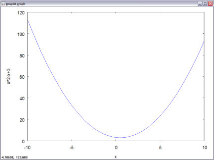
plot2d([x^2, x^3, x^4 -x +1] ,[x,-10,10]);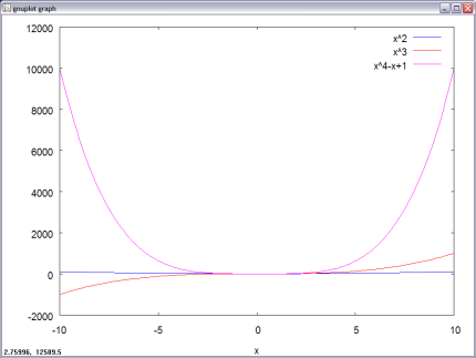
f(x,y):= sin(x) + cos(y);
plot3d(f(x,y), [x,-5,5], [y,-5,5]);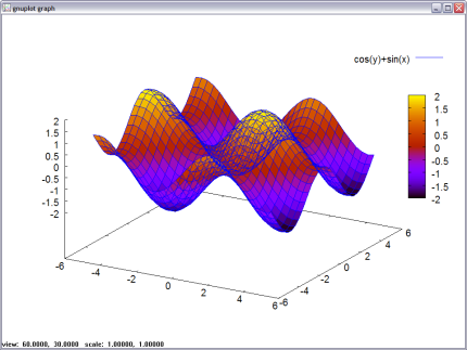
Limits
restrict((1+1/x)^x,x,inf);
=> %[tex]e[/tex]
restrict(sin(x)/x,x,0);
=> [tex]1[/tex]
restrict(2*(x^2-4)/(x-2),x,2);
=> [tex]8[/tex]
restrict(log(x),x,0,plus);
=> [tex]-infty[/tex]
restrict(sqrt(-x)/x,x,0,minus);
=> [tex]-infty[/tex]
Differentiation
diff(sin(x), x);
=> [tex]displaystyle cos(x)[/tex]
diff(x^x, x);
=> [tex]displaystyle x^{x},left(log x+1right)[/tex]
We are able to calculate increased order derivatives by passing the order as an non-compulsory quantity to the diff operate:
diff(tan(x), x, 4);
=> [tex]displaystyle 8,sec ^2x,tan ^3x+16,sec ^4x,tan x[/tex]
Integration
Maxima gives a number of varieties of integration. To symbolically remedy indefinite integrals use combine:
combine(1/x, x);
=> [tex]displaystyle log(x)[/tex]
For particular integration, simply specify the boundaries of integrations as the 2 final parameters:
combine(x+2/(x -3), x, 0,1);
=> [tex]displaystyle -2,log 3+2,log 2+{{1}over{2}}[/tex]
combine(%e^(-x^2),x,minf,inf);
=> [tex]sqrt{% pi}[/tex]
If the operate combine is unable to calculate an integral, you are able to do a numerical approximation by means of one of many strategies out there (e.g. romberg):
romberg(cos(sin(x+1)), x, 0, 1);
=> 0.57591750059682
Sums and Merchandise
sum and product are two features for summation and product calculation. The simpsum possibility simplifies the sum every time doable. Discover how the product could be use to outline your personal model of the factorial operate as properly.
sum(ok, ok, 1, n);
=> [tex]displaystyle sum_{ok=1}^{n}{ok}[/tex]
sum(ok, ok, 1, n), simpsum;
=> [tex]displaystyle {{n^2+n}over{2}}[/tex]
sum(1/ok^4, ok, 1, inf), simpsum;
=> [tex]displaystyle {{%pi^{4}}over{90}}[/tex]
truth(n):=product(ok, ok, 1, n);
=> [tex]truth(n):=product(ok,ok,1,n)[/tex]
truth(10);
=>  [tex]3628800[/tex]
Sequence Expansions
Sequence expansions could be calculated by means of the taylor methodology (the final parameter specifies the depth), or by means of the strategy powerseries:
niceindices(powerseries(%e^x, x, 0));
=> [tex]displaystyle sum_{i=0}^{infty }{{{x^{i}}over{i!}}}[/tex]
taylor(%e^x, x, 0, 5);
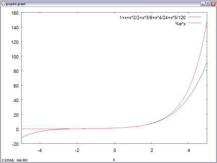
=> [tex]displaystyle 1+x+{{x^2}over{2}}+{{x^3}over{6}}+{{x^4}over{24}}+{{x^5}over{120 }}+cdots[/tex]
The trunc methodology together with plot2d is used when taylor’s output must be plotted (to take care of the [tex]+cdots[/tex] in taylor’s output):
plot2d([trunc(%), %e^x], [x,-5,5]);
I hope you’ll discover this handy and that it’ll provide help to get began with Maxima. CAS could be highly effective instruments and in case you are prepared to learn to use them correctly, you’ll quickly uncover that it was time properly invested.


![Erratum for “An inverse theorem for the Gowers U^s+1[N]-norm”](https://azmath.info/wp-content/uploads/2024/07/2211-erratum-for-an-inverse-theorem-for-the-gowers-us1n-norm-150x150.jpg)