Prediction may be very troublesome, particularly in regards to the future.
Frequent citation, variously attributed to Yogi Berra, Niels Bohr, Mark Twain and others.
Introduction
In Isaac Asimov’s well-known science fiction novel Basis, a gaggle of scientists within the distant future led by Hari Seldon uncover a mathematical technique to foretell the course of future occasions, anticipating the collapse of the reigning Galactic Empire into a brand new Darkish Age. Armed with the mathematical strategies of Hari Seldon’s “psychohistory,” the scientists create a Basis on the sting of the Galaxy that saves civilization from the prophesied Darkish Age. The notion that arithmetic can be utilized to foretell human conduct in economics, finance, politics, and plenty of different fields and actions has nice enchantment. With the unfold of more and more highly effective computer systems, complicated mathematical fashions of economics, finance, and different human actions have turn out to be increasingly more frequent. Typically, the motives are a lot much less admirable than the selfless tremendous scientists of Asimov’s story. Typically, too, the accuracy and efficiency of the mathematical fashions has been a lot much less spectacular than Asimov’s fictional new science of psychohistory.
In the previous few years, complicated fashions of the worth of mortgage backed securities have confirmed disastrously incorrect, a significant contributing issue to the Nice Recession, the current monetary disaster. That is solely the most recent in a succession of such failures in quantitative finance. Equally, many refined econometric fashions of the financial system have confirmed unreliable. To the extent that these fashions are shaping public coverage, private and company funding selections, and so forth, the pitfalls of mathematical modeling and seemingly abstruse points within the philosophy of science equivalent to Karl Popper‘s doctrine of falsifiability are having a considerable impression on individuals and society.
In actual fact, making use of mathematical fashions to economics, finance, and different human actions is particularly treacherous. All mathematical modeling suffers from the deep downside that one can assemble an infinite vary of capabilities that approximate present observations and information arbitrarily nicely and but make any and all attainable predictions about attainable new observations. In observe, human beings use varied criterion to pick out mathematical fashions which are prone to be true, lots of which criterion can’t be justified in any rigorous or rational approach and a few of which criterion are troublesome to establish (instinct, “that simply doesn’t really feel proper”, “God doesn’t play cube with the universe.”). Nonetheless, human judgment has a excessive error price, although certainly far more correct than a blind guess.
Along with this pervasive downside, most of the assumptions utilized in making use of mathematical fashions to bodily processes such because the movement of the planets or radioactive decay certainly don’t apply to economics, finance, or different types of human conduct. Our expectation is that the movement of the planets is ruled by the identical “legal guidelines” immediately as final 12 months or final decade or in 1605 when Johannes Kepler first acknowledged the elliptical orbits of the planets. Certainly, this regularity of many pure phenomenon is strongly born out by expertise. Then again, the financial system or monetary markets or different human actions change and evolve. Nonetheless imperfectly, human beings study from errors, develop new applied sciences and processes. Human beings are herd animals and vulnerable to fads and fashions that don’t have any parallel in bodily phenomena. One wouldn’t anticipate the marketplace for gold to be the identical immediately as in 1960 and it was not. The worth of gold was mounted by the US federal authorities in 1960 and immediately it isn’t.
This text takes a have a look at the value of gold since 1970 when america ended the gold normal. Gold is at the moment rising sharply in value because it did within the late 1970’s and early 1980’s. This text will present how it’s attainable to assemble many alternative purely symbolic mathematical fashions of the value of gold that make completely different predictions. Certainly, one can cook dinner up no matter prediction one would love. The article will even talk about the intense issues with making use of the mathematical strategies of physics and different “exhausting” sciences to the value of gold as a selected instance of a normal downside.
Arithmetic for Goldfinger
With the collapse of the Bretton-Woods international change system (1968-1971), the value of gold, beforehand mounted to the US greenback, was allowed to drift free. Since 1970 the value of an oz. of gold in US {dollars} has risen considerably.
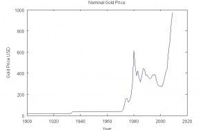
Nominal Gold Worth
America authorities reviews a client value index (CPI) that’s presupposed to mirror the price of dwelling in US {dollars} for a typical US citizen. Though there are some causes to be skeptical in regards to the accuracy of the CPI in recent times, this text will use the CPI as a proxy for the general value stage in america.
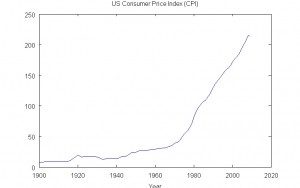
United States Client Worth Index
One can see that the CPI has usually risen at a better price since america ended the gold normal in 1970. This additionally corresponds to a interval of general rising power costs and really restricted progress in energy and propulsion applied sciences. Many different areas have seen comparatively restricted scientific and technological progress throughout this era. Computer systems and electronics have, in fact, continued their historic pattern of speedy progress to the current.
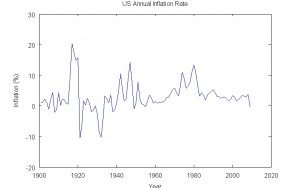
Traditionally, the US inflation price was excessive throughout the intervals of World Struggle I and World Struggle II, however in any other case usually decrease than the current interval, since 1970. The official inflation price, the speed of enhance of the CPI, was particularly excessive throughout the Nineteen Seventies, a interval of sharp will increase in nominal and actual power costs. The inflation price derived from the CPI in recent times doesn’t appear to mirror the frequent expertise of rising power costs for the reason that late Nineties. Nor does it present any proof of the sharp rise in housing costs within the US from 2002 to 2005; by many estimates, housing costs in city areas stay excessive in comparison with the historic pattern.
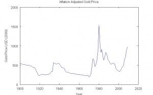
Inflation Adjusted Gold Worth
Traders are usually taken with the actual inflation-adjusted worth of an funding. The worth of gold in actual phrases fluctuated considerably throughout the interval of the gold normal however has fluctuated far more since 1970. Notably notable is the massive spike in the actual and nominal value of gold within the early 1980’s. In actual phrases, the present rise in gold value has not reached the extent of the spike within the early 1980’s. If inflation has been larger than the official CPI, the present actual value of gold could be even decrease than the spike within the early Eighties.
One can assemble a easy symbolic mathematical mannequin of the actual value of gold since 1970 (the gold normal disintegrated between 1968 and August 1971 when the US authorities ended any try to tie the greenback to gold) through the use of a polynomial with a number of phrases:
[tex] [mathrm{p}left( tright) =c,{t}^{2}+b,t+a] [/tex]
The place [tex]mathrm{p}left( tright)[/tex] is the gold value as a operate of the time [tex]t[/tex]. This can be a easy mathematical mannequin with little real-world justification. It can, in actual fact, make grossly unrealistic predictions that ought to name it into query. A polynomial mannequin of the time collection of actual gold costs is:
[tex] [mathrm{p}left( tright) =l,{t}^{11}+k,{t}^{10}+j,{t}^{9}+i,{t}^{8}+h,{t}^{7}][/tex]
[tex][ + g,{t}^{6}+f,{t}^{5}+e,{t}^{4}+d,{t}^{3}+c,{t}^{2}+b,t+a][/tex]
Polynomial Mannequin of Gold Worth (12 Phrases)
One can approximate any steady operate as precisely as one would love with a sum of a collection of powers. The issue is {that a} energy equivalent to [tex] t^{12} [/tex] will develop with out certain because the impartial variable [tex] t [/tex] grows. That is often fairly unrealistic. This can be a easy illustration of the distinction between a symbolic mathematical mannequin of actuality and our frequent sense day by day sense of actuality.
Apocalypse or Gold Bubble?
Many different mathematical fashions are attainable. In actual fact, there are an infinite variety of capabilities or curves that agree with the info throughout the interval from 1970 to 2009. On this approach, one can predict something. In mathematical fashions of bodily phenomenon, it’s common to attempt to assemble the mannequin from a set of constructing block capabilities, or extra usually phrases equivalent to phrases in a differential equation. This can be arbitrary or justified by arguing that the constructing blocks signify basic constructing blocks of the bodily course of in a roundabout way. In observe, one is attempting to seize regularities within the information that will recur in new information. For instance, the place of a pendulum is periodic; it repeats time and again. Easy harmonic movement of this kind was one of many first sorts of conduct understood mathematically by the ancients. One can assemble fashions of the gold value information that agree with the info fairly nicely by eye utilizing a set of peaks quite than periodic capabilities. One would possibly, for instance, signify the seeming peaks within the gold value information because the Gaussian or Regular operate, generally known as the “Bell Curve,”
[tex][ N(t, mu, sigma) = frac{1.0}{sqrt{2pi},sigma} {{e}^{-frac{1.0,{left( t-muright) }^{2}}{{sigma}^{2}}} }][/tex]
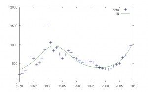
A quite simple mannequin is the sum of two Gaussians:
[tex] [mathrm{p}left( tright) = A_1N(t,mu_1,sigma_1) + A_2 N(t, mu_2, sigma_2) ] [/tex]
Gold 2 Gaussian Mannequin
This straightforward mannequin with two Gaussians doesn’t agree very nicely with the info. It predicts the next future efficiency:
Gold 2 Gaussian Prediction
It predicts that the actual value of gold will peak in about 2025 after which drop. One can get significantly better settlement between the mannequin and the gold value information by including extra Gaussians, loosely comparable to the obvious gold peaks in about 1974, 1982, 1987, 1993, and immediately. The spike in 1982 is particularly sharp and might higher be approximated by combining two Gaussians.
Gold 7 Gaussian Mannequin
Now the settlement by eye is significantly better. The curves seem basically the identical. This mannequin makes a unique prediction.
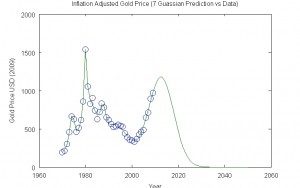
Gold 7 Gaussian Prediction
This mannequin predicts a peak in actual gold costs in only a few years, about 2012, adopted by a decline to basically zero. One can get considerably completely different predictions just by utilizing a unique operate to mannequin the peaks within the gold value. For instance, one can use the Cauchy-Lorentz distribution as a mannequin for the peaks:
[tex][mathrm{C}left( t,mu,sigmaright) =frac{1}{frac{{left( x-muright) }^{2}}{{sigma}^{2}}+1}][/tex]
the place [tex]t[/tex] is the time (12 months on this case), [tex] mu [/tex] is the placement of the height, and [tex] sigma [/tex] is a measure of the width or dispersion of the height. Initially, one can attempt a mannequin with two peaks:
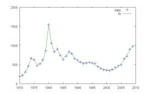
[tex] [mathrm{p}left( tright) = A_1C(t,mu_1,sigma_1) + A_2 C(t, mu_2, sigma_2) ] [/tex]
Gold 2 Cauchy Mannequin
This mannequin appears similar to the 2 Gaussian mannequin. It predicts one thing completely different nevertheless.
Gold 2 Cauchy Prediction
On this case, the value of gold trails off slowly as an alternative of dropping to basically zero in a couple of decade. This can be a distinction between the Gaussian and the Cauchy-Lorentz capabilities. In fact, the settlement between the mannequin and information will not be excellent. One in all probability wouldn’t and mustn’t belief it. One can obtain higher settlement with extra peaks, simply as within the Gaussian fashions.
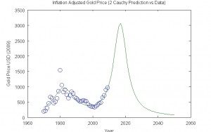
Gold 7 Cauchy Mannequin
Now the settlement is nearly precise by eye. The prediction nevertheless differs from the seven Gaussian mannequin.
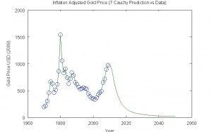
Gold 7 Cauchy Prediction
Once more, the value of gold trails off slowly over a interval of many years as a result of distinction between the Gaussian and Cauchy-Lorentz peak fashions. In actual fact, one can get basically any prediction by selecting the suitable mathematical mannequin. How cheap are these predictions? There are a number of theories in regards to the current rise in gold costs. One clear contender is that the gold value rise within the final decade is one more speculative monetary bubble. On this state of affairs, one would anticipate the value of gold to drop considerably inside a decade. One may also argue that the sharp run-up in gold costs will encourage overproduction of gold and the event of higher gold refining, recycling applied sciences, alternate options to gold, and even maybe the alchemist’s dream of changing base metals into gold (utilizing nuclear reactors for instance). On the different excessive, the rise in gold costs is tied to apocalyptic situations wherein the US and different governments go bankrupt as a consequence of deficit spending and the greenback and different paper currencies turns into as worthless because the German mark throughout the notorious German hyperinflation. Thus, the actual inflation-adjusted value of gold spikes as traders search an inflation proof haven. Sadly, civilization collapses. Gold and different luxurious objects turn out to be worthless within the bitter Darwinian battle for survival within the post-apocalyptic world. Probably the most worthwhile possessions are a gun, ammunition, and a big horde of dried meals — all bought from advertisers on Alex Jones website. In both state of affairs, gold ultimately tanks.
All kidding apart, it’s often attainable to search out technically refined, believable justifications for mathematical fashions. Often doesn’t imply at all times. The conduct of the polynomial fashions is grossly unrealistic. How possible is it that the value of gold would go detrimental, not to mention extraordinarily detrimental — that means that folks could be paying giant sums of cash to eliminate gold? The proof that the Earth is almost spherical with a diameter of about 8000 miles may be very robust. Any argument that the Earth is absolutely flat is extraordinarily troublesome to make within the current day. Most of us are fairly assured that the Solar will set immediately and rise once more tomorrow and proceed to take action for a lot of, a few years to return. There may be some data that’s fairly sure. There are some mathematical fashions which have confirmed extraordinarily correct and dependable.
Nonetheless, it’s often attainable to search out believable arguments for mathematical fashions and conceptual theories. One can often clarify away even grossly contradictory — “falsifying” within the language of Karl Popper — observations or experiments in a technically refined, believable approach. This may create the phantasm {that a} principle or mathematical mannequin falls into the class of virtually sure data, our frequent sense notion of a reality. As soon as upon a time, many individuals believed that it was a indisputable fact that the Earth was flat. How may it probably be a sphere? Political energy, social standing, and sizable funding are inclined to stream to those that declare certainty, to know exhausting info quite than speculative theories. In frequent pondering, an professional is somebody who says “I do know the reply.” not somebody who says “I don’t know.”
Scientists and science popularizers typically search to advertise reigning scientific theories to the extent of “virtually sure” data or “info,” equivalent to that the Earth is roughly spherical or the historic reality of the Holocaust. These latter two are the most typical analogies cited within the well-liked science literature. Scientific theories are mentioned to be supported by “overwhelming proof.” There’s a “consensus” that the idea is appropriate. The speculation is now not a principle, however a reality. In debates about evolution and creation, one encounters the curious declare that evolution is a falsifiable principle, that creationism or “clever design” will not be falsifiable and thus not scientific, and that evolution can also be a reality past any cheap dispute or falsification. More and more, malcontents or die-hards who query the “consensus” are “deniers” or “denialists” in analogy to Holocaust deniers, an especially emotional analogy certainly. There at the moment are evolution deniers, AIDS deniers, international warming deniers, and a rising record of different deniers. But, sure data is comparatively uncommon particularly within the frontiers of science.
Within the case of gold, one could make a robust argument that the fashions above are unlikely to be appropriate. There’s a sure basic demand for gold for industrial makes use of, in electronics for instance. There’s a lengthy historical past of individuals shopping for gold for jewellery. The financial and political issues, the fears and the greed, which have traditionally pushed the fluctuations within the value of gold are prone to proceed via the twenty first century. Thus, one ought to doubt fashions that present the actual value of gold dropping to zero or practically zero. But, each symbolic arithmetic and verbal reasoning allow one to make a believable argument that it will occur, supported by fancy symbolic arithmetic and technical graphs.
A Deep Downside
It’s at all times attainable to completely match or match any set of [tex]N[/tex] information factors utilizing a linear mixture of a minimum of [tex]N[/tex] linearly impartial capabilities. Underneath many circumstances, a operate or composition of constructing block capabilities with [tex]N[/tex] adjustable parameters also can match or match any set of [tex]N[/tex] information factors. As well as, with creativity and trial and error, one can typically assemble mathematical fashions with lower than [tex]N[/tex] parameters or constructing block capabilities that nonetheless do an excellent job of matching or becoming [tex]N[/tex] information factors. These fashions might typically fail to foretell future information or information that lies exterior of the area used to make the mannequin or match.
Typically, a composition of a set of constructing block capabilities has a type of plasticity, a sure capacity to match any information to some extent. If there are [tex]N[/tex] constructing block capabilities or adjustable parameters and [tex]N[/tex] information factors, this plasticity might be rigorously proven to be basically infinite, that’s the mannequin can at all times match any set of [tex]N[/tex] information factors. The thinker of science Karl Popper known as such fashions or theories unfalsifiable. They will by no means be confirmed fallacious. They predict every little thing and due to this fact in addition they predict nothing. In contrast to well-liked displays of his doctrine of falsifiability, Popper acknowledged that falsifiability was typically not a black and white distinction. There have been levels of falsifiability and he tried to outline some logical and quantitative criterion for the diploma of falsifiability. What this implies is {that a} mathematical mannequin or principle with [tex]M[/tex] adjustable parameters the place [tex]M[/tex] is lower than the variety of information factors [tex]N[/tex] should still match a broad class of attainable observations or information. It may be falsified, maybe, however solely with nice issue. There may be, within the examples above, a number of freedom to match many alternative units of information with seven peaks within the mannequin. The fashions have 21 adjustable parameters and there are 40 information factors (40 years). Though the fashions can’t precisely match all units of 40 information factors, nonetheless they’re prone to be ok for many functions. Remaining variations between the info and the fashions can simply be attributed to noise, measurement errors, or some related excuse.
In physics, there are some examples of very giant information units that match quite simple mathematical formulation. The motions of the planets within the Photo voltaic System conform to Kepler’s Legal guidelines and Newton’s principle of gravitation to a really excessive diploma. This isn’t essentially true for the movement of stars within the Milky Manner galaxy, galaxies in galactic clusters and so forth. A deviation from Newtonian gravity is a attainable rationalization for the anomalies typically cited as proof for so-called “darkish matter” or “darkish power.” So too, there is a gigantic quantity of quantitative information on the vibration of springs and strings, the movement of pendulums, easy radioactive decays, and varied different bodily phenomena that present exact matches to easy mathematical expressions equivalent to Hooke’s Legislation for springs or exponential decay for radioactive decay. It’s truthful to say that the quantity of information factors is now within the hundreds of thousands or extra and the fashions have only some adjustable parameters such because the half-life of a radioactive isotope. Consequently, it’s in all probability cheap to have a excessive diploma of confidence in these fashions. On the different excessive, it’s clear that we must always put no confidence within the predictive energy of fashions with as many adjustable parameters or constructing block capabilities because the variety of information factors.
In lots of conditions nevertheless together with the frontiers of human data and infrequently areas like economics, the state of affairs falls right into a grey space. The theories, each symbolic mathematical fashions and conceptual fashions, could also be complicated, however not so complicated as to be clearly “unfalsifiable.” The quantity of information could also be restricted or of questionable high quality, however nonetheless not clearly insufficient to attract conclusions. It’s right here that defective human judgment is in observe utilized, partially as a result of human judgment, fallible although it undoubtedly is, remains to be the most suitable choice, extra dependable than symbolic arithmetic or laptop applications in lots of circumstances. In establishing mathematical fashions in these circumstances, human judgment is usually hidden within the definition of the symbols and the selection of constructing block capabilities or different mathematical parts used within the mannequin.
Economics, finance, politics and different human actions are particularly treacherous areas for mathematical modeling. The mathematical and scientific strategies utilized in physics and different “exhausting” sciences have been developed to check extremely repeatable phenomena that don’t seem to vary appreciably over time. For instance, a “truthful” coin will come up heads when flipped on common half the time, tails half the time. This was true within the early days of chance and statistics throughout the Renaissance. It’s true immediately. Honest video games of likelihood work the identical approach immediately as yesterday, final 12 months, final century, and presumably 1000’s of years in the past or sooner or later. One can acquire huge quantities of information on these video games. Equally, bodily phenomena such because the movement of the planets, radioactive decay, and so forth seem to behave the identical approach time after time. They don’t evolve, study from errors, neglect classes realized, or all of a sudden change for obscure causes. None of that is true of a lot financial or monetary information.
Within the instance of gold, the conduct of gold modified radically from 1968 to August 1971 when the gold normal ended. Since 1970, there have been intensive political, financial, and technological adjustments that in all probability impact the value of gold. The Chilly Struggle ended. Apartheid in gold producing South Africa ended, adopted by a big exodus of the white minority who dominated the mining business. The usage of electronics has elevated; gold is utilized in electronics. Ladies’s fashions in clothes and jewellery have modified. The terrorist assaults of September 11, 2001 in all probability contributed to normal unease and the rise in gold costs. In opposition to these many adjustments, there’s solely forty years of information on gold costs. Each day gold costs are correlated and gold appears to comply with traits over a number of years, seemingly rising and falling in peaks. Thus, there’s very restricted information to investigate in comparison with a bodily course of. On the identical time, one nonetheless has the liberty to assemble many alternative mathematical fashions, theoretically an infinite quantity.
This capacity to assemble many alternative fashions that agree with observations or experiment however which make fairly completely different predictions will not be an issue distinctive to symbolic mathematical fashions. Somewhat, we encounter the identical or an identical downside in on a regular basis life, in politics, in private relationships, the place ideas, phrases, and footage are the norm quite than symbolic arithmetic with its phantasm of certainty. It happens when opposing attorneys are capable of current radically completely different interpretations of the identical proof in a court docket case. It happens when political activists clarify the identical occasions in radically completely different ways in which virtually at all times verify their beliefs. It happens in disputes between co-workers the place every sees the identical occasion or downside fairly in another way (it’s all your fault). It happens in conflicts between husbands and wives when every sees the identical occasions in another way. If verbal ideas and psychological footage are literally mathematical fashions maintained within the mind (however not in a symbolic approach), then it could be precisely the identical downside as that encountered in mathematical modeling.
There is no such thing as a doubt that human judgment is defective and restricted. In some comparatively uncommon circumstances arithmetic or formal logic can clearly outperform human judgment. Nonetheless, in lots of conditions, human judgment and instinct nonetheless win out over arithmetic, formal logic, or laptop applications. It stays an unsolved and maybe unsolvable downside to discover a approach to choose the appropriate mannequin that, in actual fact, predicts new observations as nicely and even higher than human judgment.
The character and origin of human judgment and instinct stays an enigma. Governments have spent billions of {dollars} and many years on synthetic intelligence within the largely futile effort to duplicate even generally seemingly easy features of human reasoning. Human beings typically can’t clarify both verbally or in symbolic logical or mathematical methods their profitable reasoning processes. Historic students and philosophers would possibly attribute their concepts to divine inspiration or mystical perception. Certainly historic accounts of innovations and discoveries are replete with reported sudden insights or realizations such because the well-known story of Archimedes in his bathtub all of a sudden realizing how you can decide the gold content material of the King’s crown with out destroying the crown after which racing bare via the streets of Syracuse shouting “Heureka!” One might marvel what Archimedes feared the King would do to him if he had failed to unravel the issue. The trendy scientific view would in all probability attribute this capacity of the human thoughts to search out the appropriate reply to an anthropic or evolutionary trigger. Our mind incorporates billions of years of evolution and is thus tuned to the mysterious underlying logical or mathematical construction of the universe.
Conclusion
You will need to notice that one can assemble an infinite variety of mathematical fashions that match a set of information. In some sense, one can assemble a good “bigger” variety of mathematical fashions that match a set of information “nicely sufficient,” the place remaining variations can simply be attributed to noise, instrument error, or minor results that may be ignored for sensible functions. In highschool and faculty, one is usually uncovered to arithmetic and geometry as a rigorous deductive system. The epitome of that is Euclid’s geometry which many individuals are uncovered to in highschool; highschool math programs usually train the primary three of Euclid’s 13 books. One begins with axioms and definitions that always appear self-evident, with the attainable exception of the so-called parallel postulate. One can apply a sequence of logical steps to get a exact unambiguous reply. Equally, highschool and faculty science programs steadily focus totally on extraordinarily well-measured phenomena equivalent to vibrating springs or radioactive decay that exactly comply with easy mathematical legal guidelines. Scientists are sometimes described as “deriving,” “determining,” or “deducing” mathematical legal guidelines equivalent to Newton’s Idea of Gravitation, Maxwell’s Equations of Electromagnetism, or Schrodinger’s Equation for quantum mechanics. The implication is that these mathematical theories might be discovered by the appliance of rigorous mathematical or logical guidelines, a lot in the way in which that theorems in Euclidean geometry are confirmed. This has an ideal enchantment in comparison with messy, fallible human judgment and instinct. However the actuality is that the theories have been discovered via the appliance of messy, fallible human judgment and instinct, maybe assisted by some arithmetic, by mannequin becoming strategies, and so forth, however ultimately it was mysterious human judgment and instinct.
If we may perceive what human beings are literally doing, this is able to be an ideal advance. It might be a good larger advance to discover a approach to enhance human judgment and instinct, which is actually fairly fallible.
Within the meantime, it’s significantly hazardous to attempt to apply mathematical modeling to economics, finance, and human conduct. This doesn’t imply that we must always not attempt. Nor does it imply that there might not be successes in making use of arithmetic to human exercise. Certainly, in economics, there are some mathematical guidelines of thumb which are typically appropriate. It’s, for instance, usually noticed that inflation is decrease when unemployment is larger; this relation loosely follows a mathematical curve. Nonetheless, we’re a really lengthy distance from a predictive mathematical technique similar to Isaac Asimov’s fictional psychohistory if that is even attainable. Most individuals don’t assume in arithmetic; can human conduct actually be decreased to arithmetic?
The current monetary disaster illustrates that these seemingly abstruse problems with mathematical fashions can impression the lives of many individuals and organizations. That is, if something, prone to enhance with rising reliance on computer systems and mathematical fashions applied in laptop software program and {hardware}. There stays no larger knowledge than the traditional Latin saying: Caveat Emptor (Purchaser Beware).
Observe: An appendix with the technical particulars of the evaluation and plots offered above follows the Urged Studying/References part under. This consists of the uncooked information, the fashions, and the Octave scripts used to suit the fashions to the annual gold value information. This text is primarily for informational and academic functions. It isn’t funding recommendation.
Copyright © 2010 John F. McGowan, Ph.D.
Concerning the Creator
John F. McGowan, Ph.D. is a software program developer, analysis scientist, and guide. He works primarily within the space of complicated algorithms that embody superior mathematical and logical ideas, together with speech recognition and video compression applied sciences. He has intensive expertise creating software program in C, C++, Visible Fundamental, Mathematica, MATLAB, and plenty of different programming languages. He’s in all probability finest identified for his AVI Overview, an Web FAQ (Continuously Requested Questions) on the Microsoft AVI (Audio Video Interleave) file format. He has labored as a contractor at NASA Ames Analysis Heart concerned within the analysis and improvement of picture and video processing algorithms and know-how. He has revealed articles on the origin and evolution of life, the exploration of Mars (anticipating the invention of methane on Mars), and low cost entry to house. He has a Ph.D. in physics from the College of Illinois at Urbana-Champaign and a B.S. in physics from the California Institute of Know-how (Caltech). He might be reached at [email protected].
Urged Studying/References
Karl Popper, The Logic of Scientific Discovery, Routledge, London, England 2000 (First revealed 1959, English translation with new notes and appendices of Logik der Forschung, revealed Vienna, Austria, 1934)
Paul Feyerabend, In opposition to Methodology (third Version), Verso, 1993
Thomas Kuhn, The Construction of Scientific Revolutions, College Of Chicago Press; third version (December 15, 1996)
John D. Barrow and Frank J. Tipler, The Anthropic Cosmological Precept, Oxford College Press, New York, 1986
Isaac Asimov, Basis, Spectra; Revised version (October 1, 1991)
Roger Lowenstein, When Genius Failed: The Rise and Fall of Lengthy Time period Capital Administration, Random Home, New York, 2000
Emanuel Derman, My Life as a Quant: Reflections on Physics and Finance, John Wiley and Sons, Hoboken, New Jersey, 2004
Charles MacKay, Extraordinary Well-liked Delusions and the Insanity of Crowds, Farrar, Straus, and Giroux, New York, 1932 (first revealed in London in 1841)
Robert J. Shiller, Irrational Exuberance, Broadway Books, New York, 2000
Dean Baker, False Income: Recovering from the Bubble Financial system, Polipoint Press (January 15, 2010)
Michael Specter, Denialism: how irrational pondering hinders scientific progress, harms the planet, and threatens our lives, Penguin Press, 2009
Seth C. Kalichman, Denying AIDS: Conspiracy Theories, Pseudoscience, and Human Tragedy, Springer, 2009
Invoice McKibben, “Sizzling Mess: Why are conservatives so radical about local weather?”, The New Republic, October 6, 2010
Appendix: Technical Particulars
The annual gold value information used on this article is from the World Gold Council. Right here is the precise uncooked information.
1900    20.67    4.25        o    1900    8.14    0.037941643    544.78            1913-01-01    0.10
1901    20.67    4.25        o    1901    8.24    0.038407756    538.17            1913-01-02    0.10
1902    20.67    4.25        o    1902    8.34    0.03887387    531.72            1913-01-03    0.10
1903    20.67    4.25        o    1903    8.53    0.039759485    519.88            1913-01-04    0.10
1904    20.67    4.25        o    1904    8.63    0.040225599    513.85            1913-01-05    0.10
1905    20.67    4.25        o    1905    8.53    0.039759485    519.88            1913-01-06    0.10
1906    20.67    4.25        o    1906    8.72    0.040645101    508.55            1913-01-07    0.10
1907    20.67    4.25        o    1907    9.11    0.042462944    486.78            1913-01-08    0.10
1908    20.67    4.25        o    1908    8.92    0.041577328    497.15            1913-01-09    0.10
1909    20.67    4.25        o    1909    8.82    0.041111215    502.78            1913-01-10    0.10
1910    20.67    4.25        o    1910    9.21    0.042929058    481.49            1913-01-11    0.10
1911    20.67    4.25        o    1911    9.21    0.042929058    481.49            1913-01-12    0.10
1912    20.67    4.25        o    1912    9.4    0.043814673    471.76            1914-01-01    0.10
1913    20.67    4.25        12/31/1913    1913    9.6    0.04630723    446.37    10        1914-01-02    0.10
1914    20.67    4.25        12/31/1914    1914    9.69    0.046770302    441.95    10.1        1914-01-03    0.10
1915    20.67    4.25        12/31/1915    1915    9.74    0.047696447    433.37    10.3        1914-01-04    0.10
1916    20.67    4.25        12/31/1916    1916    10.64    0.053716387    384.80    11.6        1914-01-05    0.10
1917    20.67    4.25        12/31/1917    1917    12.82    0.063440905    325.82    13.7        1914-01-06    0.10
1918    20.67    4.25        12/31/1918    1918    15.06    0.076406929    270.53    16.5        1914-01-07    0.10
1919    20.67    4.50        12/31/1919    1919    17.3    0.087520665    236.17    18.9        1914-01-08    0.10
1920    20.67    5.60        12/31/1920    1920    20.04    0.089836026    230.09    19.4        1914-01-09    0.10
1921    20.67    5.35        12/31/1921    1921    17.9    0.080111508    258.02    17.3        1914-01-10    0.10
1922    20.67    4.69        12/31/1922    1922    16.77    0.078259219    264.12    16.9        1914-01-11    0.10
1923    20.67    4.51        12/31/1923    1923    17.07    0.080111508    258.02    17.3        1914-01-12    0.10
1924    20.67    4.68        12/31/1924    1924    17.1    0.080111508    258.02    17.3        1915-01-01    0.10
1925    20.67    4.25        12/31/1925    1925    17.53    0.082889942    249.37    17.9        1915-01-02    0.10
1926    20.67    4.25        12/31/1926    1926    17.7    0.081963797    252.18    17.7        1915-01-03    0.10
1927    20.67    4.25        12/31/1927    1927    17.37    0.080111508    258.02    17.3        1915-01-04    0.10
1928    20.67    4.25        12/31/1928    1928    17.13    0.079185363    261.03    17.1        1915-01-05    0.10
1929    20.67    4.25        12/31/1929    1929    17.13    0.079648436    259.52    17.2        1915-01-06    0.10
1930    20.67    4.25        12/31/1930    1930    16.7    0.07455464    277.25    16.1        1915-01-07    0.10
1931    20.67    4.25        12/31/1931    1931    15.23    0.067608556    305.73    14.6        1915-01-08    0.10
1932    20.67    5.90        12/31/1932    1932    13.66    0.060662471    340.74    13.1        1915-01-09    0.10
1933    20.67    6.24        12/31/1933    1933    12.96    0.061125544    338.16    13.2        1915-01-10    0.10
1934    35.00    6.88        12/31/1934    1934    13.39    0.062051688    564.05    13.4        1915-01-11    0.10
1935    35.00    7.11        12/31/1935    1935    13.73    0.063903977    547.70    13.8        1915-01-12    0.10
1936    35.00    7.02        12/31/1936    1936    13.86    0.064830122    539.87    14        1916-01-01    0.10
1937    35.00    7.04        12/31/1937    1937    14.36    0.066682411    524.88    14.4        1916-01-02    0.10
1938    35.00    7.13        12/31/1938    1938    14.09    0.064830122    539.87    14        1916-01-03    0.11
1939    35.00    7.72        12/31/1939    1939    13.89    0.064830122    539.87    14        1916-01-04    0.11
1940    35.00    8.40        12/31/1940    1940    14.03    0.065293194    536.04    14.1        1916-01-05    0.11
1941    35.00    8.40        12/31/1941    1941    14.73    0.071776206    487.63    15.5        1916-01-06    0.11
1942    35.00    8.40        12/31/1942    1942    16.3    0.078259219    447.23    16.9        1916-01-07    0.11
1943    35.00    8.40        12/31/1943    1943    17.3    0.08057458    434.38    17.4        1916-01-08    0.11
1944    35.00    8.40        12/31/1944    1944    17.6    0.082426869    424.62    17.8        1916-01-09    0.11
1945    35.00    8.61        12/31/1945    1945    18    0.084279159    415.29    18.2        1916-01-10    0.11
1946    35.00    8.61        12/31/1946    1946    19.54    0.099560544    351.54    21.5        1916-01-11    0.12
1947    35.00    8.61        12/31/1947    1947    22.34    0.108358918    323.00    23.4        1916-01-12    0.12
1948    35.00    8.68        12/31/1948    1948    24.08    0.111600424    313.62    24.1        1917-01-01    0.12
1949    35.00    9.40        12/31/1949    1949    23.85    0.109285063    320.26    23.6        1917-01-02    0.12
1950    35.00    12.50        12/31/1950    1950    24.08    0.115768075    302.33    25        1917-01-03    0.12
1951    35.00    12.50        12/31/1951    1951    25.98    0.122714159    285.22    26.5        1917-01-04    0.13
1952    35.00    12.50        12/31/1952    1952    26.55    0.123640304    283.08    26.7        1917-01-05    0.13
1953    35.00    12.50        12/31/1953    1953    26.75    0.124566449    280.97    26.9        1917-01-06    0.13
1954    35.00    12.50        12/31/1954    1954    26.88    0.123640304    283.08    26.7        1917-01-07    0.13
1955    35.00    12.50        12/31/1955    1955    26.78    0.124103376    282.02    26.8        1917-01-08    0.13
1956    35.00    12.50        12/31/1956    1956    27.18    0.127807955    273.85    27.6        1917-01-09    0.13
1957    35.00    12.50        12/31/1957    1957    28.15    0.131512533    266.13    28.4        1917-01-10    0.14
1958    35.00    12.50        12/31/1958    1958    28.92    0.133827895    261.53    28.9        1917-01-11    0.14
1959    35.00    12.50        12/31/1959    1959    29.16    0.136143256    257.08    29.4        1917-01-12    0.14
1960    35.00    12.50        12/31/1960    1960    29.62    0.137995545    253.63    29.8        1918-01-01    0.14
1961    35.00    12.50        12/31/1961    1961    29.92    0.13892169    251.94    30        1918-01-02    0.14
1962    35.00    12.50        12/31/1962    1962    30.26    0.140773979    248.63    30.4        1918-01-03    0.14
1963    35.00    12.50        12/31/1963    1963    30.62    0.143089341    244.60    30.9        1918-01-04    0.14
1964    35.00    12.50        12/31/1964    1964    31.03    0.144478557    242.25    31.2        1918-01-05    0.15
1965    35.00    12.50        12/31/1965    1965    31.56    0.147256991    237.68    31.8        1918-01-06    0.15
1966    35.00    12.50        12/31/1966    1966    32.46    0.152350787    229.73    32.9        1918-01-07    0.15
1967    35.00    12.65        12/31/1967    1967    33.4    0.15698151    222.96    33.9        1918-01-08    0.15
1968    38.94    16.23        12/31/1968    1968    34.8    0.164390666    236.87    35.5        1918-01-09    0.16
1969    40.76    16.98        12/31/1969    1969    36.67    0.174578257    233.48    37.7        1918-01-10    0.16
1970    36.07    15.03        12/31/1970    1970    38.84    0.184302775    195.71    39.8        1918-01-11    0.16
1971    41.17    16.91        12/31/1971    1971    40.51    0.190322715    216.32    41.1        1918-01-12    0.17
1972    59.00    23.58        12/31/1972    1972    41.85    0.196805727    299.79    42.5        1919-01-01    0.17
1973    97.84    39.90        12/31/1973    1973    44.45    0.213939402    457.33    46.2        1919-01-02    0.16
1974    158.96    67.96        12/31/1974    1974    49.33    0.240334523    661.41    51.9        1919-01-03    0.16
1975    160.91    72.42        12/31/1975    1975    53.84    0.257005126    626.10    55.5        1919-01-04    0.17
1976    124.71    69.05        12/31/1976    1976    56.94    0.269508078    462.73    58.2        1919-01-05    0.17
1977    147.78    84.66        12/31/1977    1977    60.61    0.287567898    513.90    62.1        1919-01-06    0.17
1978    193.39    100.75        12/31/1978    1978    65.22    0.313499947    616.87    67.7        1919-01-07    0.17
1979    304.83    143.68        12/31/1979    1979    72.57    0.355176454    858.25    76.7        1919-01-08    0.18
1980    614.61    264.20        12/31/1980    1980    82.38    0.399631394    1537.94    86.3        1919-01-09    0.18
1981    459.26    226.47        12/31/1981    1981    90.93    0.435287962    1055.07    94        1919-01-10    0.18
1982    375.28    214.38        12/31/1982    1982    96.5    0.451958564    830.34    97.6        1919-01-11    0.19
1983    423.61    279.24        12/31/1983    1983    99.6    0.469092239    903.04    101.3        1919-01-12    0.19
1984    360.50    269.77        12/31/1984    1984    103.9    0.487615131    739.31    105.3        1920-01-01    0.19
1985    317.18    244.68        12/31/1985    1985    107.6    0.506138023    626.67    109.3        1920-01-02    0.20
1986    367.72    250.66        12/31/1986    1986    109.6    0.511694891    718.63    110.5        1920-01-03    0.20
1987    446.28    272.30        12/31/1987    1987    113.6    0.534385434    835.13    115.4        1920-01-04    0.20
1988    436.79    245.20        12/31/1988    1988    118.3    0.558002121    782.77    120.5        1920-01-05    0.21
1989    380.74    232.20        12/31/1989    1989    124    0.58393417    652.03    126.1        1920-01-06    0.21
1990    383.32    214.78        12/31/1990    1990    130.7    0.619590737    618.67    133.8        1920-01-07    0.21
1991    362.10    204.65        12/31/1991    1991    136.2    0.638576701    567.04    137.9        1920-01-08    0.20
1992    343.86    194.76        12/31/1992    1992    140.3    0.657099593    523.30    141.9        1920-01-09    0.20
1993    360.00    239.68        12/31/1993    1993    144.5    0.675159413    533.21    145.8        1920-01-10    0.20
1994    384.12    250.79        12/31/1994    1994    148.2    0.693219232    554.11    149.7        1920-01-11    0.20
1995    384.05    243.31        12/31/1995    1995    152.4    0.71081598    540.29    153.5        1920-01-12    0.19
1996    387.82    248.33        12/31/1996    1996    156.9    0.734432667    528.05    158.6        1921-01-01    0.19
1997    330.98    202.10        12/31/1997    1997    160.5    0.746935619    443.12    161.3        1921-01-02    0.18
1998    294.12    177.56        12/31/1998    1998    163    0.758975499    387.52    163.9        1921-01-03    0.18
1999    278.55    172.13        12/31/1999    1999    166.6    0.77935068    357.41    168.3        1921-01-04    0.18
2000    279.10    184.09        12/31/2000    2000    172.2    0.805745801    346.39    174        1921-01-05    0.18
2001    272.67    189.36        12/31/2001    2001    177.1    0.818248753    333.24    176.7        1921-01-06    0.18
2002    309.66    206.27        12/31/2002    2002    179.9    0.83769779    369.66    180.9        1921-01-07    0.18
2003    362.91    222.20        12/31/2003    2003    184    0.853442248    425.23    184.3        1921-01-08    0.18
2004    409.17    223.36        12/31/2004    2004    188.9    0.881226586    464.32    190.3        1921-01-09    0.18
2005    444.47    244.86        12/31/2005    2005    195.3    0.911326285    487.72    196.8        1921-01-10    0.18
2006    603.95    327.68        12/31/2006    2006    201.6    0.9344799    646.30    201.8        1921-01-11    0.17
2007    695.39    347.00        12/31/2007    2007    207.34    0.972618535    714.96    210.036        1921-01-12    0.17
2008    871.65    473.17        12/31/2008    2008    215.3    0.973507634    895.37    210.228        1922-01-01    0.17
2009    972.90    621.59        12/31/2009    2009    214.54    1    972.90    215.949        1922-01-02    0.17
The fashions have been fitted to the info utilizing the free Octave numerical programming setting. Octave is Matlab suitable and accessible beneath the GNU Public License. Octave is on the market in binary in addition to supply code variations for Home windows, Mac OS, and Linux. The usual polyfit polynomial becoming operate in Octave was used to suit the polynomial fashions to the annual gold value information. The leasqr least squares becoming operate from the optim Octave add-on bundle was used to suit the Gaussian and Cauchy-Lorentz peak fashions to the annual gold value information. Octave Forge add-on packages can be found as Unix type blatz.tar.gz information. There is no such thing as a have to extract the contents of those information. Octave has a command pkg set up which handles putting in the packages; simply sort pkg set up blatz.tar.gz. The GNU Octave set up features a C/C++ compiler to compile any C or C++ information included within the bundle. Observe that the run-time errors reported by Octave, for instance as a consequence of a syntax error, might be cryptic. Be affected person and don’t at all times belief the error message.
% plot_gold.m
% Description: Octave (Matlab suitable) script to plot annual gold value information
% and match polynomial fashions to the info.  Examined on Home windows XP Service Pack 2
% with Octave 3.2.4 for Home windows put in.
%
% Creator: John F. McGowan, Ph.D.
% Copyright (C) 2010 by John F. McGowan
%
%
disp('studying gold value information...');
fflush(stdout);
information = dlmread('annual_gold_price_from_1900.txt');
disp('making plot 1');
fflush(stdout);
determine(1)
plot(information(:,1), information(:,8));
title('Inflation Adjusted Gold Worth');
xlabel('12 months');
ylabel('Gold Worth USD (2009)');
disp('making plot 2');
fflush(stdout);
determine(2)
plot(information(:,1), information(:,2));
title('Nominal Gold Worth');
xlabel('12 months');
ylabel('Gold Worth USD');
disp('making cpi plot');
determine(3)
plot(information(:,1), information(:,6));
title('US Client Worth Index (CPI)');
xlabel('12 months');
% annual inflation price
disp('plotting annual inflation price');
fflush(stdout);
determine(4)
cpi = information(:,6);
cpi_shift = shift(cpi,1);
inflation = (cpi - cpi_shift) ./ cpi_shift;
years = information(:,1);
plot(years(2:finish), inflation(2:finish)*100);
title('US Annual Inflation Price');
xlabel('12 months');
ylabel('Inflation (%)');
%
% becoming polynomial mannequin to information 1970 to 2009
%
disp('making gold value prediction 12 phrases');
fflush(stdout);
determine(5)
floating = years(71:finish);
floating_gold_price = information(71:finish, 8);
p = polyfit(floating, floating_gold_price, 12);
prediction = (1970:2020);
f = polyval(p, prediction);
plot(floating, floating_gold_price, 'o', prediction, f, '-');
title('Polynomial Mannequin of Gold Worth (12 Phrases)');
xlabel('12 months');
ylabel('Gold Worth USD (2009)');
%
disp('making gold value prediction 24 phrases');
fflush(stdout);
determine(6)
floating = years(71:finish);
floating_gold_price = information(71:finish, 8);
p = polyfit(floating, floating_gold_price, 24);
prediction = (1970:2020);
f = polyval(p, prediction);
plot(floating, floating_gold_price, 'o', prediction, f, '-');
title('Polynomial Mannequin of Gold Worth (24 Phrases)');
xlabel('12 months');
ylabel('Gold Worth USD (2009)');
%
disp('making gold value prediction 32 phrases');
fflush(stdout);
determine(7)
floating = years(71:finish);
floating_gold_price = information(71:finish, 8);
p = polyfit(floating, floating_gold_price, 32);
prediction = (1970:2020);
f = polyval(p, prediction);
plot(floating, floating_gold_price, 'o', prediction, f, '-');
title('Polynomial Mannequin of Gold Worth (32 Phrases)');
xlabel('12 months');
ylabel('Gold Worth USD (2009)');
disp('all finished');
fflush(stdout);

% THE END
The script to suit the 2 Gaussian peak mannequin to the info is:
% fit_gold.m
% Description: Octave (matlab suitable) script to suit two gaussian peak mannequin
% to annual gold value information utilizing Octave 3.2.4 and the optim bundle model 1.0.15
% Examined on Home windows XP Service Pack 2 with Octave 3.2.4 and optim 1.0.15 put in.
%
% Creator: John F. McGowan, Ph.D.
% Copyright (C) 2010 by John F. McGowan
%
disp('becoming mannequin to gold value information');
fflush(stdout);
% match mannequin to gold value information
%floating_gold_price has inflation adjusted gold value since 1970
floating_years = years(71:finish);

% Outline capabilities
% mannequin annual gold value information as two Gaussians
leasqrfunc = @(x,p) p(1) * exp(-1.0*(x - p(2)).^2/p(3)^2) + p(4) * exp(-1.0*(x - p(5)).^2/p(6)^2);
leasqrdfdp = @(x, f, p, dp, func) [exp(-1.0*(x - p(2)).^2/p(3)^2), (2*(x - p(2))/p(3)^2) * p(1) .* exp(-1.0*(x - p(2)).^2/p(3)^2), (2 * (x - p(2)).^2/p(3)^3) * p(1) .* exp(-1.0*(x - p(2)).^2/p(3)^2), exp(-1.0*(x - p(5)).^2/p(6)^2), (2*(x - p(5))/p(6).^2) * p(4) .* exp(-1.0*(x - p(5)).^2/p(6)^2), (2 * (x - p(5)).^2/p(6)^3) * p(4) .* exp(-1.0*(x - p(5)).^2/p(6)^2) ];

wt1 = ones(dimension(floating_gold_price));
t = floating_years;
information = floating_gold_price;

F = leasqrfunc;
dFdp = leasqrdfdp; % precise spinoff
dp = [50.0; 1.0; 1.0; 50.0; 1.0; 1.0];
pin = [500.0; 1980.; 5.0; 500.0; 2010.0; 5.0 ];
stol=0.01; niter=50;
minstep = [10.0; 0.2; 0.2; 10.0; 0.2; 0.2];
maxstep = [100.0; 5.0; 5.0; 100.0; 5.0; 5.0];
choices = [minstep, maxstep];

disp(dimension(t));
disp(dimension(information));
disp(dimension(wt1));
fflush(stdout);
determine(1);
international verbose;
verbose = 1;
[f1, p1, kvg1, iter1, corp1, covp1, covr1, stdresid1, Z1, r21] = ...
leasqr (t, information, pin, F, stol, niter, wt1, dp, dFdp, choices);

%
% make a prediction
determine(2);
pred_years = [1970:2020];
prediction = leasqrfunc(pred_years, p1);
plot(floating_years, information, 'o', pred_years, prediction, '-');
title('Inflation Adjusted Gold Worth (Prediction vs Information)');
xlabel('12 months');
ylabel('Gold Worth USD (2009)');
%
determine(3);
pred_years = [1970:2050];
prediction = leasqrfunc(pred_years, p1);
plot(floating_years, information, 'o', pred_years, prediction, '-');
title('Inflation Adjusted Gold Worth (Prediction vs Information)');
xlabel('12 months');
ylabel('Gold Worth USD (2009)');
%
determine(4);
pred_years = [1970:2100];
prediction = leasqrfunc(pred_years, p1);
plot(floating_years, information, 'o', pred_years, prediction, '-');
title('Inflation Adjusted Gold Worth (Prediction vs Information)');
xlabel('12 months');
ylabel('Gold Worth USD (2009)');

data_2G = information;
model_2G = leasqrfunc(floating_years, p1);
diff_2G = model_2G - data_2G;
chisq_2G = diff_2G' * diff_2G;

disp('all finished');
% THE END
The script to suit the seven (7) Gaussian peak mannequin to the annual gold value information is:
% fit_gold7.m
% Description: Octave (matlab suitable) script to suit seven (7) Gaussian peak mannequin
% to annual gold value information.
% Examined utilizing Octave 3.2.4 with optim 1.0.15 add on bundle put in on Home windows XP Service Pack 2
% Creator: John F. McGowan, Ph.D.
% Copyright (C) John F. McGowan
%
disp('becoming 7 Gaussian mannequin to gold value information');
fflush(stdout);
% match mannequin to gold value information
%floating_gold_price has inflation adjusted gold value since 1970
floating_years = years(71:finish);

% Outline capabilities

% mannequin as seven (7) un-normalized Gaussians
leasqrfunc = @(x,p) p(1) * exp(-1.0*(x - p(2)).^2/p(3)^2) + p(4) * exp(-1.0*(x - p(5)).^2/p(6)^2) + p(7) * exp(-1.0*(x - p(8)).^2/p(9)^2) + p(10) * exp(-1.0*(x - p(11)).^2/p(12)^2) + p(13) * exp(-1.0*(x - p(14)).^2/p(15)^2) + p(16) * exp(-1.0*(x - p(17)).^2/p(18)^2) + p(19) * exp(-1.0*(x - p(20)).^2/p(21)^2);

leasqrdfdp = @(x, f, p, dp, func) [exp(-1.0*(x - p(2)).^2/p(3)^2), (2*(x - p(2))/p(3)^2) * p(1) .* exp(-1.0*(x - p(2)).^2/p(3)^2), (2 * (x - p(2)).^2/p(3)^3) * p(1) .* exp(-1.0*(x - p(2)).^2/p(3)^2), exp(-1.0*(x - p(5)).^2/p(6)^2), (2*(x - p(5))/p(6).^2) * p(4) .* exp(-1.0*(x - p(5)).^2/p(6)^2), (2 * (x - p(5)).^2/p(6)^3) * p(4) .* exp(-1.0*(x - p(5)).^2/p(6)^2), exp(-1.0*(x - p(8)).^2/p(9)^2), (2*(x - p(8))/p(9)^2) * p(7) .* exp(-1.0*(x - p(8)).^2/p(9)^2), (2 * (x - p(8)).^2/p(9)^3) * p(7) .* exp(-1.0*(x - p(8)).^2/p(9)^2) , exp(-1.0*(x - p(11)).^2/p(12)^2), (2*(x - p(11))/p(12)^2) * p(10) .* exp(-1.0*(x - p(11)).^2/p(12)^2), (2 * (x - p(11)).^2/p(12)^3) * p(10) .* exp(-1.0*(x - p(11)).^2/p(12)^2) , exp(-1.0*(x - p(14)).^2/p(15)^2), (2*(x - p(14))/p(15)^2) * p(13) .* exp(-1.0*(x - p(14)).^2/p(15)^2), (2 * (x - p(14)).^2/p(15)^3) * p(13) .* exp(-1.0*(x - p(14)).^2/p(15)^2), exp(-1.0*(x - p(17)).^2/p(18)^2), (2*(x - p(17))/p(18)^2) * p(16) .* exp(-1.0*(x - p(17)).^2/p(18)^2), (2 * (x - p(17)).^2/p(18)^3) * p(16) .* exp(-1.0*(x - p(17)).^2/p(18)^2) , exp(-1.0*(x - p(20)).^2/p(21)^2), (2*(x - p(20))/p(21)^2) * p(19) .* exp(-1.0*(x - p(20)).^2/p(21)^2), (2 * (x - p(20)).^2/p(21)^3) * p(19) .* exp(-1.0*(x - p(20)).^2/p(21)^2) ];

wt1 = ones(dimension(floating_gold_price));
t = floating_years;
information = floating_gold_price;

F = leasqrfunc;
dFdp = leasqrdfdp; % precise spinoff
dp = [50.0; 1.0; 1.0; 50.0; 1.0; 1.0; 50.0; 1.0; 1.0; 50.0; 1.0; 1.0 ; 50.0; 1.0; 1.0; 50.0; 1.0; 1.0; 50.0; 1.0; 1.0];
pin = [500.0; 1980.; 5.0; 500.0; 2010.0; 5.0; 500.0; 1982; 2.0; 500.0; 1987; 2.0; 500.0; 1995; 5.0 ; 500.0; 1974; 5.0; 500.0; 1974; 5.0 ];
stol=0.01; niter=100;
minstep = [10.0; 0.2; 0.2; 10.0; 0.2; 0.2; 10.0; 0.2; 0.2; 10.0; 0.1; 0.1; 10.0; 0.1; 0.1; 10.0; 0.1; 0.1; 10.0; 0.1; 0.1];
maxstep = [100.0; 5.0; 5.0; 100.0; 5.0; 5.0; 100.0; 5.0; 5.0; 100.0; 5.0; 5.0; 100.0; 5.0; 5.0; 100.0; 5.0; 5.0; 100.0; 5.0; 5.0];
choices = [minstep, maxstep];

disp(dimension(t));
disp(dimension(information));
disp(dimension(wt1));
fflush(stdout);
determine(1);
international verbose;
verbose = 1;
[f1, p1, kvg1, iter1, corp1, covp1, covr1, stdresid1, Z1, r21] = ...
leasqr (t, information, pin, F, stol, niter, wt1, dp, dFdp, choices);

%
% make a prediction
determine(2);
pred_years = [1970:2020];
prediction = leasqrfunc(pred_years, p1);
plot(floating_years, information, 'o', pred_years, prediction, '-');
title('Inflation Adjusted Gold Worth (7 Gaussian Prediction vs Information)');
xlabel('12 months');
ylabel('Gold Worth USD (2009)');
%
determine(3);
pred_years = [1970:2050];
prediction = leasqrfunc(pred_years, p1);
plot(floating_years, information, 'o', pred_years, prediction, '-');
title('Inflation Adjusted Gold Worth (7 Guassian Prediction vs Information)');
xlabel('12 months');
ylabel('Gold Worth USD (2009)');
%
determine(4);
pred_years = [1970:2100];
prediction = leasqrfunc(pred_years, p1);
plot(floating_years, information, 'o', pred_years, prediction, '-');
title('Inflation Adjusted Gold Worth (7 Gaussian Prediction vs Information)');
xlabel('12 months');
ylabel('Gold Worth USD (2009)');

data_7G = information;
model_7G = leasqrfunc(floating_years, p1);
diff_7G = model_7G - data_7G;
chisq_7G = diff_7G' * diff_7G;

disp('all finished (7 Gaussian Match) all finished');
% THE END
The script to suit the 2 Cauchy-Lorentz operate peak mannequin to the annual gold value information is:
% fit_gold_cauchy.m
% Description: Octave (matlab suitable) script to suit a two Cauchy-Lorentz peak mannequin to the annual gold value information.  Examined utilizing Octave 3.2.4 and the optim 1.015 add-on bundle on Home windows XP Service Pack 2.
% Creator: John F. McGowan, Ph.D.
% Copyright (C) John F. McGowan
%
disp('becoming 2 Cauchy-Lorentz mannequin to gold value information');
fflush(stdout);
% match mannequin to gold value information
%floating_gold_price has inflation adjusted gold value since 1970
floating_years = years(71:finish);

% Outline capabilities

% mannequin because the linear mixture of two Cauchy-Lorentz (aka Breit-Wigner) capabilities
leasqrfunc = @(x,p) p(1) ./(1 + (x - p(2)).^2/p(3)^2) + p(4) ./(1 + (x - p(5)).^2/p(6)^2);
leasqrdfdp = @(x, f, p, dp, func) [1.0 ./(1.0 + (x - p(2)).^2/p(3)^2), (2*p(1)*(x-p(2)))./(p(3)^2*((x-p(2)).^2/p(3)^2+1).^2), (2*p(1)*(x-p(2)).^2)./(p(3)^3*((x-p(2)).^2/p(3)^2+1).^2), 1.0 ./(1.0 + (x - p(5)).^2/p(6)^2), (2*p(4)*(x-p(5)))./(p(6)^2*((x-p(5)).^2/p(6)^2+1).^2), (2*p(4)*(x-p(5)).^2)./(p(6)^3*((x-p(5)).^2/p(6)^2+1).^2)];

wt1 = ones(dimension(floating_gold_price));
t = floating_years;
information = floating_gold_price;

F = leasqrfunc;
dFdp = leasqrdfdp; % precise spinoff
dp = [50.0; 1.0; 1.0; 50.0; 1.0; 1.0];
pin = [500.0; 1980.; 5.0; 500.0; 2010.0; 5.0 ];
stol=0.01; niter=50;
minstep = [10.0; 0.2; 0.2; 10.0; 0.2; 0.2];
maxstep = [100.0; 5.0; 5.0; 100.0; 5.0; 5.0];
choices = [minstep, maxstep];

disp(dimension(t));
disp(dimension(information));
disp(dimension(wt1));
fflush(stdout);
determine(1);
international verbose;
verbose = 1;
[f1, p1, kvg1, iter1, corp1, covp1, covr1, stdresid1, Z1, r21] = ...
leasqr (t, information, pin, F, stol, niter, wt1, dp, dFdp, choices);

%
% make a prediction
determine(2);
pred_years = [1970:2020];
prediction = leasqrfunc(pred_years, p1);
plot(floating_years, information, 'o', pred_years, prediction, '-');
title('Inflation Adjusted Gold Worth (2 Cauchy Prediction vs Information)');
xlabel('12 months');
ylabel('Gold Worth USD (2009)');
%
determine(3);
pred_years = [1970:2050];
prediction = leasqrfunc(pred_years, p1);
plot(floating_years, information, 'o', pred_years, prediction, '-');
title('Inflation Adjusted Gold Worth (2 Cauchy Prediction vs Information)');
xlabel('12 months');
ylabel('Gold Worth USD (2009)');
%
determine(4);
pred_years = [1970:2100];
prediction = leasqrfunc(pred_years, p1);
plot(floating_years, information, 'o', pred_years, prediction, '-');
title('Inflation Adjusted Gold Worth (2 Cauchy Prediction vs Information)');
xlabel('12 months');
ylabel('Gold Worth USD (2009)');

% C suffix for Cauchy Lorentz mannequin
data_2C = information;
model_2C = leasqrfunc(floating_years, p1);
diff_2C = model_2C - data_2C;
chisq_2C = diff_2C' * diff_2C;

disp('all finished');
% THE END
The Octave script to suit the seven (7) Cauchy-Lorentz peak mannequin to the annual gold value information is:
% fit_gold7.m
% Description: Octave (matlab suitable) script to suit seven (7) Cauchy-Lorentz peak mannequin
% to annual gold value information.
% Examined utilizing Octave 3.2.4 with optim 1.0.15 add on bundle put in on Home windows XP Service Pack 2
% Creator: John F. McGowan, Ph.D.
% Copyright (C) John F. McGowan
%
disp('becoming seven (7) Cauchy-Lorentz mannequin to gold value information');
fflush(stdout);
% match mannequin to gold value information
%floating_gold_price has inflation adjusted gold value since 1970
floating_years = years(71:finish);

% Outline gold value mannequin capabilities

% mannequin as linear mixture of seven (7) Cauchy-Lorentz (aka Breit-Wigner) capabilities
leasqrfunc = @(x,p) p(1) ./(1 + (x - p(2)).^2/p(3)^2) + p(4) ./(1 + (x - p(5)).^2/p(6)^2) + p(7) ./(1 + (x - p(8)).^2/p(9)^2) + p(10) ./(1 + (x - p(11)).^2/p(12)^2) + p(13) ./(1 + (x - p(14)).^2/p(15)^2) + p(16) ./(1 + (x - p(17)).^2/p(18)^2) + p(19) ./(1 + (x - p(20)).^2/p(21)^2);

leasqrdfdp = @(x, f, p, dp, func) [1.0 ./(1.0 + (x - p(2)).^2/p(3)^2), (2*p(1)*(x-p(2)))./(p(3)^2*((x-p(2)).^2/p(3)^2+1).^2), (2*p(1)*(x-p(2)).^2)./(p(3)^3*((x-p(2)).^2/p(3)^2+1).^2),1.0 ./(1.0 + (x - p(5)).^2/p(6)^2), (2*p(4)*(x-p(5)))./(p(6)^2*((x-p(5)).^2/p(6)^2+1).^2), (2*p(4)*(x-p(5)).^2)./(p(6)^3*((x-p(5)).^2/p(6)^2+1).^2),1.0 ./(1.0 + (x - p(8)).^2/p(9)^2), (2*p(7)*(x-p(8)))./(p(9)^2*((x-p(8)).^2/p(9)^2+1).^2), (2*p(7)*(x-p(8)).^2)./(p(9)^3*((x-p(8)).^2/p(9)^2+1).^2),1.0 ./(1.0 + (x - p(11)).^2/p(12)^2), (2*p(10)*(x-p(11)))./(p(12)^2*((x-p(11)).^2/p(12)^2+1).^2), (2*p(10)*(x-p(11)).^2)./(p(12)^3*((x-p(11)).^2/p(12)^2+1).^2),1.0 ./(1.0 + (x - p(14)).^2/p(15)^2), (2*p(13)*(x-p(14)))./(p(15)^2*((x-p(14)).^2/p(15)^2+1).^2), (2*p(13)*(x-p(14)).^2)./(p(15)^3*((x-p(14)).^2/p(15)^2+1).^2),1.0 ./(1.0 + (x - p(17)).^2/p(18)^2), (2*p(16)*(x-p(17)))./(p(18)^2*((x-p(17)).^2/p(18)^2+1).^2), (2*p(16)*(x-p(17)).^2)./(p(18)^3*((x-p(17)).^2/p(18)^2+1).^2),1.0 ./(1.0 + (x - p(20)).^2/p(21)^2), (2*p(19)*(x-p(20)))./(p(21)^2*((x-p(20)).^2/p(21)^2+1).^2), (2*p(19)*(x-p(20)).^2)./(p(21)^3*((x-p(20)).^2/p(21)^2+1).^2)]

wt1 = ones(dimension(floating_gold_price));  % identical weight for all information factors
t = floating_years;    % years when gold value floats
information = floating_gold_price;   % inflation adjusted gold value

F = leasqrfunc;
dFdp = leasqrdfdp; % precise spinoff
dp = [50.0; 1.0; 1.0; 50.0; 1.0; 1.0; 50.0; 1.0; 1.0; 50.0; 1.0; 1.0 ; 50.0; 1.0; 1.0; 50.0; 1.0; 1.0; 50.0; 1.0; 1.0];
pin = [500.0; 1980.; 5.0; 500.0; 2010.0; 5.0; 500.0; 1982; 2.0; 500.0; 1987; 2.0; 500.0; 1995; 5.0 ; 500.0; 1974; 5.0; 500.0; 1974; 5.0 ];
stol=0.01; niter=100;
minstep = [10.0; 0.2; 0.2; 10.0; 0.2; 0.2; 10.0; 0.2; 0.2; 10.0; 0.1; 0.1; 10.0; 0.1; 0.1; 10.0; 0.1; 0.1; 10.0; 0.1; 0.1];
maxstep = [100.0; 5.0; 5.0; 100.0; 5.0; 5.0; 100.0; 5.0; 5.0; 100.0; 5.0; 5.0; 100.0; 5.0; 5.0; 100.0; 5.0; 5.0; 100.0; 5.0; 5.0];
choices = [minstep, maxstep];

disp(dimension(t));
disp(dimension(information));
disp(dimension(wt1));
fflush(stdout);
determine(1);
international verbose;
verbose = 1;
[f1, p1, kvg1, iter1, corp1, covp1, covr1, stdresid1, Z1, r21] = ...
leasqr (t, information, pin, F, stol, niter, wt1, dp, dFdp, choices);

%
% make a prediction
determine(2);
pred_years = [1970:2020];
prediction = leasqrfunc(pred_years, p1);
plot(floating_years, information, 'o', pred_years, prediction, '-');
title('Inflation Adjusted Gold Worth (7 Cauchy Prediction vs Information)');
xlabel('12 months');
ylabel('Gold Worth USD (2009)');
%
determine(3);
pred_years = [1970:2050];
prediction = leasqrfunc(pred_years, p1);
plot(floating_years, information, 'o', pred_years, prediction, '-');
title('Inflation Adjusted Gold Worth (7 Cauchy Prediction vs Information)');
xlabel('12 months');
ylabel('Gold Worth USD (2009)');
%
disp('plotting determine 4');
fflush(stdout);
determine(4);
pred_years = [1970:2100];
prediction = leasqrfunc(pred_years, p1);
plot(floating_years, information, 'o', pred_years, prediction, '-');
title('Inflation Adjusted Gold Worth (7 Cauchy Prediction vs Information)');
xlabel('12 months');
ylabel('Gold Worth USD (2009)');

disp('computing closing outcomes...');
fflush(stdout);
% C suffix for Cauchy Lorentz mannequin
data_7C = information;
model_7C = leasqrfunc(floating_years, p1);
diff_7C = model_7C - data_7C;
chisq_7C = diff_7C' * diff_7C;

disp('all finished');
% THE END
The derivatives of the fashions with respect to parameters have been computed with the symbolic manipulation bundle Maxima. Maxima was additionally used to generate a number of the Latex mathematical formulation on this article.


![Erratum for “An inverse theorem for the Gowers U^s+1[N]-norm”](https://azmath.info/wp-content/uploads/2024/07/2211-erratum-for-an-inverse-theorem-for-the-gowers-us1n-norm-150x150.jpg)